
Executive Summary
Our Two-Step Modeling Solution is designed to neutralize the potential appeals tsunami at the front gate, decoupling value generation from value certification:
Step 1: Sales-Based Valuation Modeling (The Genesis): Establishes a foundational econometric model by optimizing sales-sample data to achieve Best Linear Unbiased Estimator (BLUE) status, producing a highly accurate Tentative Roll (the theme of our prior Forensic Valuation Modeling series/book).
Step 2: Population-Based Equalization Modeling (The Clean-up): The core mechanism of this session. Instead of blindly certifying the Tentative Roll, Step 2 executes a population-level audit of the jurisdiction’s own generated Just Values. It intercepts, isolates, and scrubs out systemic inconsistencies and administrative distortions before the roll is finalized. This proactive approach is the best defense against horizontal inequity and costly appeals and litigations.
Session 3 extends the Champ-Challenger framework from administrative boundaries (Sessions 1–2) to a major market fault line: Coastal vs. Non-Coastal towns.
Using a Coastal County dataset with two coastal and two non-coastal towns, we simulate a direct contest between the Coastal towns (Champion) and Non-Coastal towns (Challengers). With 9 Zip Codes for location control, we apply the same disciplined 2-Pass Equalization Valuation Modeling approach.
A striking finding in this session is that the Homestead variable remains negative in Pass 2 (–$2,119). With 16,270 non-homesteaded properties in the dataset, this could shift valuations by approximately $49 million across these four towns alone. When extrapolated to all 12 towns in the County, the exposure could be manifold higher. This is a prime example of the financial and legal risks assessing offices face when population-level distortions are left unaddressed.
The Champ-Challenger Just Value Ratio (JVR) comparison reveals meaningful differences in how Coastal and Non-Coastal areas are valued. These insights provide assessing offices with a powerful preventative diagnostic while giving Review Commissions, VABs, and consultants independent forensic evidence to enforce horizontal equity.
For Assessing Staff: This is your pre-certification stress test — the best way to strengthen the tentative roll and avoid the appeals tsunami.
For Oversight Bodies and Consultants: This is your transparent verification standard when issues need to be challenged.
Session 3 proves that only by deploying Step 2 Population Equalization can administrators expose and flatten these localized town-level disparities, guiding taxing jurisdictions away from catastrophic litigation and onto the true path to administrative Nirvana.
Deep-Dive Introduction
Welcome to Session 3 of our Equalization Valuation Modeling.
Building on the administrative boundary comparisons in Sessions 1 and 2, we now extend the Champ-Challenger framework to a major market fault line: Coastal vs. Non-Coastal towns.
Using a Coastal County dataset with two coastal and two similarly sized non-coastal towns, we simulate a direct contest between the Coastal towns (Champion) and Non-Coastal towns (Challengers). With 9 Zip Codes for location control, we apply the same disciplined 2-Pass Equalization Valuation Modeling approach.
What you will see:
1. How One-Step CAMA creates a tsunami — and how our Two-Step neutralizes it at the front gate.
2. The $49M Homestead exposure hiding in 4 towns — and the $147M+ liability when extrapolated county-wide.
3. The Coastal Divide — how a one-step model achieves a “perfect” 1.00 average JVR by under-assessing the waterfront and over-assessing the interior.
This session has one goal: to prove that sales accuracy is not equity in the population. And we’ll give you the protocol to fix it before VAB does.
Step 1 creates the Tentative Roll. Step 2 makes it Certifiable. Let’s walk Step 2 together.
Analysis of Regression Model (Pass 1)
(a) Data Construction & The Market Fault Line
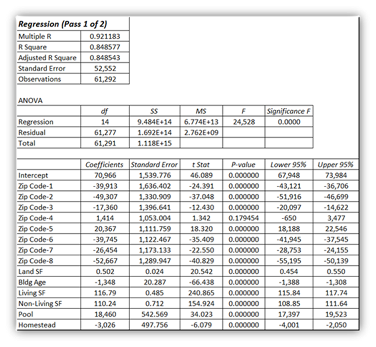
To test the structural integrity of the centralized County mass appraisal model, the dataset isolates a Coastal Florida County comprising two Coastal and two Non-Coastal towns, with 61,292 total observations.
The data was strictly pruned to isolate standard single-family residential properties and eliminate systemic noise:
· Value Floor: Removed all properties with a Just Value under $100K to avoid unverified or compromised parcels.
· Acreage Ceiling: Stripped out lots greater than 2 acres. This purposefully excludes grandfathered agricultural single-family residences (SFRs) and horse ranches, which are traditionally hand-appraised by assessment staff rather than scored by automated mass models.
· Micro-Lot Floor: Excluded extra-small lots (<2,000 SF) to maintain sample balance.
The Champ-Challenger Setup: We designate the two Coastal towns as the Champion and the two Non-Coastal towns as the Challengers. This allows us to evaluate whether the County’s mass appraisal model exhibits any systematic inequities that favor or disadvantage coastal properties. We will later compare Just Value Ratios (JVRs) between the two groups using both the County’s actual values and our model’s predictions.
Because this is an equalization model optimizing Just Value on the latest roll, time adjustments are irrelevant; all values are natively pinned to the target valuation date of January 1, 2026.
(b) Resident Stratification: The Homestead Experiment
A key feature of this session is the experimental introduction of Homestead as a binary variable (1 = {True} for permanent residents; 0 = {False} for seasonal “winter birds,” vacation properties, or investor-owned short-term rentals/Airbnbs).
The Pass 1 output reveals a statistically significant coefficient of -$3,026 for homesteaded properties. This indicates that, holding all physical features and geography constant, full-time permanent residences carry a minor downward valuation variance compared to investor-owned or seasonal properties. Non-homesteaded properties (27% of the dataset, or 16,270 homes) carry the premium, likely reflecting the aggressive market demand for turnkey vacation rentals and seasonal investments in a highly sought-after retirement destination.
(c) Macro Model Stats & The Omitted Variable Bias (OVB) Proxy
The baseline macro metrics showcase a highly significant, high-performing model that still contains hidden population-level strain:
· Explanatory Power: The R-square of 0.84857 shows that the model explains roughly 85% of the variance in County’s Just Values.
· The “Average Miss”: The Standard Error stands at $52,552. This wide margin is expected in Pass 1 due to the unscrubbed 27% non-homesteaded market variance and the presence of heavy-tailed outliers.
· Overall Significance: An F-value of 24,528 with a Significance F of 0.0000 confirms that the probability of these variables explaining the variance by pure chance is zero.
The OVB Spatial Proxy
The structural flaw of the central model is exposed by comparing structural coefficients:
· Living SF Coefficient: $116.79 per square foot.
· Non-Living SF Coefficient: $110.24 per square foot.
In a clean property model, unheated/non-living square footage (patios, screen enclosures, garages) would never carry a value nearly equal to that of the finished living space. This narrow $6.55 delta is a textbook case of Omitted Variable Bias (OVB). Because the dataset lacks an explicit, high-quality GIS View variable, the regression engine is forced to allocate the massive premium for waterfront locations to other physical variables. Non-Living SF is a proxy for luxury outdoor features—expansive lanais, wraparound decks, and premium backyards overlooking the water.
(d) Reading the Zip Code Coefficients Relative to the Intercept
The Intercept of $70,966 represents the theoretical baseline value of a property in this county, where all continuous variables (Land SF, Bldg Age, Living SF, Non-Living SF) are zero, all binary flags (Pool, Homestead) are false (0), and the property sits within the omitted Zip Code-9 reference zone.
Because Zip Code-9 is the reference baseline, the other 8 dummy-coded Zip Code coefficients must be read as direct upward or downward shifts relative to it:
· Zip Code-8 (-$52,667): Properties here are valued $52,667 less than identical properties in Zip Code-9.
· Zip Code-2 (-$49,307): Properties here carry a $49,307 discount relative to Zip Code-9.
· Zip Code-5 (+$20,367): This is our high-tier localized market zone, commanding a $20,367 premium over the Zip Code-9 baseline.
· Zip Code-4 (+$1,414): Nominally values properties slightly above the baseline, and therefore carries an insignificant P-value (> 0.05).
(e) Determining Statistical Significance & Confidence
To determine whether a coefficient is reliable or merely mathematical noise, we audit the interaction of the t-Stat, P-value, and the 95% Confidence Interval (CI):
1. The P-value & t-Stat Threshold: A variable is universally deemed statistically significant if its P-value is less than 0.05 (indicating a less than 5% probability that the relationship is random). Correspondingly, the absolute value of the t-Stat must typically exceed 1.96.
2. The 95% Confidence Interval Test: The lower and upper bounds must not straddle zero. If a confidence interval spans a negative number and a positive number, it means the true coefficient could be zero, invalidating the variable’s predictive authority.
Examining the Significance Outputs:
· Physical Variables: Bldg Age (t-stat: -66.438), Living SF (t-stat: 240.865), and Pool (t-stat: 34.023) all show P-values of 0.000000. Their confidence intervals are incredibly tight (e.g., Bldg Age depreciates reliably between -$1,388 and -$1,308 annually), proving severe structural stability.
· The Zip Code-4 Exception: Looking closely at Zip Code-4, its t-Stat is only 1.342, and its P-value is a highly insignificant 0.179454. Furthermore, its 95% Confidence Interval spans from -$650 to +$3,477. Because this interval straddles zero, the regression engine cannot definitively prove that Zip Code-4 differs mathematically from the Zip Code-9 reference zone. In Pass 1, Zip Code-4 and Zip Code-9 are statistically identical.
This lays bare the initial administrative playing field. Once we execute the outlier scrub (extracting extreme Z-scores beyond ±2) and transition to Pass 2, we will see these standard errors compress, and the true town-level market fault lines emerge.
Analysis of Regression Model (Pass 2 of 2)
Interpretation of Improvements
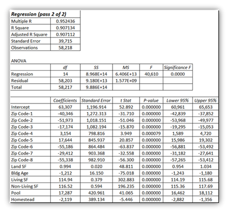
After running Pass 1 on 61,292 observations, we applied the 2-Pass Outlier Protocol (Z-scores beyond ±2). This removed approximately 5% of observations (3,074 properties), leaving a cleaner dataset of 58,218 properties for Pass 2.
· R Square improved substantially to 90.71%, meaning the model now explains roughly 91% of the variation in Just Values.
· Standard Error dropped by nearly $13K, indicating significantly more precise predictions.
· The overall model strength (F-statistic) increased dramatically.
· All coefficients retained their directional signs, and 95% confidence intervals tightened.
· Zip Code-4, which was insignificant in Pass 1, is now statistically significant with a positive coefficient and confidence interval that does not straddle zero.
Notable Findings Unique to This Session:
· Non-Living SF coefficient now exceeds Living SF ($116.52 vs. $114.94). This is a clear confirmation of Omitted Variable Bias (OVB) suspected in Pass 1. Without a View/GIS variable, Non-Living SF (lanais, patios, garages, large yards, etc.) serves as a proxy for desirable coastal amenities and views. In a properly specified model with View data, Non-Living SF should carry a significantly lower coefficient. This finding strengthens our case for disciplined variable selection and the importance of GIS data when available.
Homestead remains negative (–$2,119). This is the exact financial engine for the horizontal inequity argument. Holding all physical structures and geography equal, a permanent resident’s homesteaded property is valued at over $2,100 less than a seasonal or investor-owned property.
With thousands of such properties in the dataset, this creates meaningful exposure to horizontal inequity (similar properties treated differently based on ownership status). This is highly relevant for both assessing offices (prevention) and oversight bodies and consultants (forensic evidence for ratio challenges).
Overall Assessment: The 2-Pass Outlier Protocol delivered substantial, meaningful improvements, making the model cleaner, more precise, and more reliable. These findings — particularly the OVB with Non-Living SF and the Homestead effect — further enhance the dual-value proposition of our methodology: a preventative diagnostic tool for assessing offices and a powerful independent verification standard for VABs, Review Commissions, and consultants.
Just Value Ratio (JVR) Analysis
Just Value Ratio (JVR) Analysis: Pre- vs. Post-Outlier Removal
Reminder: JVR = Predicted Value (Model) ÷ Assessor’s Just Value
· JVR = 1.00 → Perfect alignment
· JVR > 1.00 → Assessor’s JV underestimated
· JVR < 1.00 → Assessor’s JV overestimated
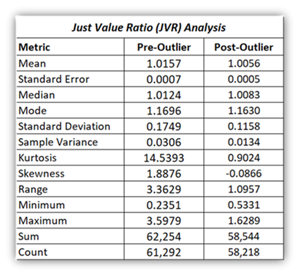
We compare the distribution of JVRs before (Pass 1: 61,292 observations) and after (Pass 2: 58,218 observations), removing ~5% outliers.
Analysis & Interpretation
1. Central Tendency: The mean JVR improved from 1.0157 to 1.0056, and the median moved closer to the ideal 1.00. This indicates better overall alignment between the model’s predictions and the County’s Just Values after outlier removal.
2. Dispersion & Uniformity: Standard Deviation dropped 34% (0.1749 → 0.1158), and variance was reduced by 56%. The extreme Range collapsed by 67% (3.36 → 1.10). These are significant improvements in uniformity across the coastal and non-coastal properties.
3. Extreme Values: The most severe over-valuations dropped from 3.5979 to 1.6289, while the worst under-valuations improved from 0.2351 to 0.5331. This cleanup removes the most distorting cases.
4. Distribution Shape (The Most Dramatic Result): Kurtosis collapsed from a high 14.54 to a near-normal 0.9024, while Skewness fell from strongly right-skewed (1.8876) to nearly symmetric (-0.0866).
This dramatic improvement once again demonstrates how a relatively small percentage of outliers (~5%) can create massive distortion in the dataset. The 2-Pass Outlier Protocol successfully restored a much cleaner, more normal distribution — reinforcing why it should be standard practice in regression-based econometric modeling for mass appraisal.
Necessary, But Not Sufficient: The Holdout Illusion
Why removing outliers during sales sample-based modeling and holdout testing is necessary but not sufficient: Removing outliers from the sales sample and achieving good holdout statistics are necessary first steps for model validation. However, it is insufficient because it does not address systemic administrative distortions, classification biases, and manual overrides that become embedded across the unsold population (the vast majority of the assessment roll). Only a disciplined 2-Pass population-level Equalization Valuation Model — which directly models the jurisdiction’s own Just Values — can provide the endurance needed to produce a tentative roll that sufficiently stands on its own with minimal bias and horizontal inequity. This is also the core advantage of the Champ-Challenger approach.
Champ-Challenger Analysis
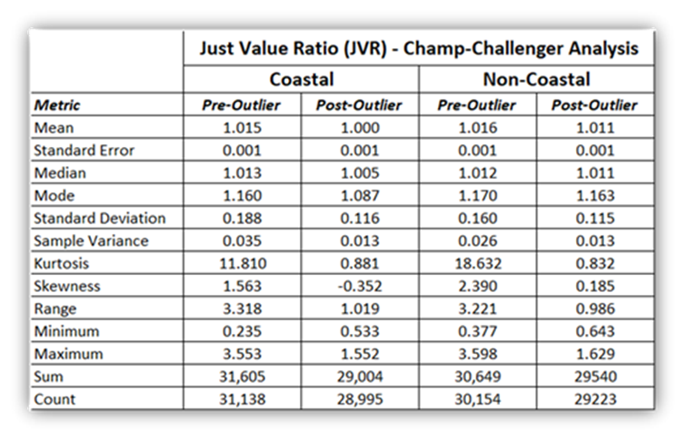
Champ (Coastal) vs. Challenger (Non-Coastal) – JVR Analysis
To provide a complete picture, we compare Pre-Outlier and Post-Outlier JVR statistics for both Coastal towns (Champion) and Non-Coastal towns (Challengers). This shows the roll in its raw state and the impact of our 2-Pass Outlier Protocol. The comparison reveals a closely contested but highly instructive result.
At first glance, the overall Post-Outlier JVR summary appears relatively clean, with a Mean near 1.00. However, when disaggregated by the critical market fault line (Coastal vs. Non-Coastal), a more concerning pattern emerges:
· The Coastal cohort (Champion) achieves near-perfect alignment (Mean JVR = 1.000, Median = 1.005).
· The Non-Coastal cohort (Challenger) shows a consistent and material upward bias (Mean = 1.011, Median = 1.011).
The Mode deviation is particularly telling: Coastal drops to 1.087, while Non-Coastal remains significantly elevated at 1.163 — indicating a large cluster of interior properties is being over-assessed by more than 16%.
Interpretation: The one-step CAMA model appears to be achieving its “average” performance through central smoothing that systematically favors coastal properties while placing a disproportionate burden on non-coastal (often inland) areas. This creates clear horizontal inequity — where similar properties are not treated equally based on location.
This is precisely why a transparent, population-level Champ-Challenger Equalization Model is so valuable: it unmasks these subtle but systemic patterns that traditional modeling and holdout testing tend to obscure.
Why our Equalization Model is the Nirvana: This 2-Pass population-level approach directly confronts the limitations of traditional one-step sales-based CAMA modeling. By modeling the entire population’s Just Values, it acts as a preventative diagnostic that helps assessment offices clean the tentative roll before finalization — dramatically reducing avoidable appeals and exposure to ratio challenges. It also gives oversight bodies and consultants independent forensic evidence when needed. This is the true Nirvana of modern mass appraisal: proactive equity instead of reactive defense.
Session Conclusion
The verdict is in. The roll is guilty.
One-Step CAMA gave you a tentative roll with Kurtosis 14.54, Max JVR 3.60, and a $49M Homestead bias. It told you the average was 1.0157 and called it a day. That’s not assessment. That’s negligence.
Two-Step Equalization gave you a certifiable roll: Kurtosis 0.90, Max JVR 1.63, and Skewness -0.09. It removed the 5% hostages, re-priced the 95% you can defend, and exposed the truth: Coastal parcels are at market. Non-Coastal parcels are 1.1% above the mean and 16.3% above the mode.
The tsunami isn’t random. It’s engineered. Your black-box engineered it by fitting it to sales and certifying it on the population without an audit. 2-Pass is the audit.
One-step CAMA built the cliff. Two-step Equalization builds the stairs.
Welcome to Equalization Modeling. Welcome to Nirvana.
Session Disclaimer
This educational series is provided for illustrative, training, and professional development purposes only. The methodologies, models, and interpretations presented should be carefully validated and adapted by qualified assessing professionals to suit the specific legal, regulatory, and market conditions of each jurisdiction. Neither the author nor the platform assumes responsibility for decisions made based on the materials in this series. Participants are encouraged to exercise professional judgment and consult with appropriate legal and valuation experts when applying these concepts in official settings.
Session 3: Frequently Asked Questions (FAQs)
Q1: What is the main focus of Session 3?
A: Session 3 moves from administrative boundaries (Sessions 1–2) to a major market fault line: Coastal vs. Non-Coastal towns. We simulate a Champ-Challenger contest to test whether the County model shows systematic inequity across this market divide.
Q2: Why do we use a Coastal County for this session?
A: Coastal vs. Non-Coastal is a fundamental market fault line that affects property values. Testing the methodology across this divide proves its robustness beyond administrative zones and shows how it can be applied to any meaningful structural or market difference.
Q3: How is the Champ-Challenger contest set up in Session 3?
A: We designate the two Coastal towns as the Champion and the two Non-Coastal towns as the Challengers. We compare their performance using Just Value Ratios (JVRs) to assess whether the model treats coastal and non-coastal properties equitably.
Q4: Why did we drop the standalone Coastal binary variable?
A: Including a Coastal binary created multicollinearity with the Zip Code dummies. Instead, we let the Zip Code dummies capture location effects for coastal value differences. This keeps the model simple, stable, and easy to explain.
Q5: What is the importance of the View/GIS data in valuation modeling?
A: View and other GIS attributes are often critical drivers of value, especially in coastal areas. Without them, variables like Non-Living SF can proxy for these missing factors (Omitted Variable Bias). When available, they should be introduced properly during initial variable selection, not added “on the fly.”
Q6: How should Assessing Offices use this methodology?
A: Assessing Offices should treat the 2-Pass Equalization Model as a pre-certification stress test and preventative shield. Running it on the tentative roll helps identify and correct loose ends before final publication, dramatically reducing avoidable appeals and ratio challenges.
Q7: How can Review Commissions, VABs, and Consultants benefit?
A: They gain an independent, transparent verification standard. If systemic issues are ignored, the Champ-Challenger analysis and “Indictment” sample provide powerful forensic evidence for data-driven ratio challenges or mass appeals.
Q8: Should foundational variables like Zip Code dummies always remain in the model?
A: Yes. Foundational variables are required by USPAP and must stay in the model regardless of statistical significance in Pass 2. We retained all Zip Code dummies even though Zip Code-4 lost significance in Pass 1 (before outlier removal) but became significant in Pass 2 (after outlier removal).
Q9: What is the Dual-Value Proposition of this approach?
A: It serves Assessing Staff as a proactive diagnostic tool to strengthen the tentative roll, while giving Oversight Bodies and Consultants a robust independent standard for verification and accountability when needed.
Q10: How does this methodology scale to larger jurisdictions?
A: The Equalization Valuation Modeling framework is platform-agnostic. Smaller and mid-sized offices can implement it effectively in Excel, while larger jurisdictions can deploy the exact same logic, variable selection discipline, and 2-Pass Outlier Protocol within their existing enterprise statistical software (SPSS, SAS, R, or Python). The core principles and diagnostic power remain consistent regardless of jurisdiction size or software platform.
Excel Steps – How to Run Regression and Descriptive Statistics in Excel (Data Analysis ToolPak)
Important: These instructions assume you are using Microsoft Excel for Windows (Excel 2010 or newer). Mac users can use the free Real Statistics Resource Pack or similar add-ins.
Step 1: Enable the Data Analysis ToolPak (One-Time Setup)
1. Open Excel and go to File → Options.
2. In the Excel Options window, select Add-ins from the left menu.
3. At the bottom, next to “Manage,” select Excel Add-ins and click Go.
4. Check the box for Analysis ToolPak (and Analysis ToolPak – VBA if available).
5. Click OK. → The Data Analysis button should now appear on the Data tab.
Step 2: Preparing Your Data for Session 3
· Dependent Variable (Y) = Just Value column
· Independent Variables (X) = 8 Zip Code dummies, Land SF, Building Age, Living SF, Non-Living SF, Bathrooms, Pool, Fireplace, Homestead
· Create a clean worksheet with only the variables you plan to use.
· Remove properties with Just Value < $100K, lots > 2 acres, and extra-small lots (< 2,000 SF) as done in the session dataset.
Step 3: Running Descriptive Statistics (for JVR Analysis)
1. Prepare your JVR column (Predicted ÷ Just Value).
2. Go to the Data tab → Click Data Analysis.
3. Select Descriptive Statistics and click OK.
4. In the dialog box:
o Input Range: Select your JVR column (including header).
o Check Labels in First Row.
o Choose an empty Output Range.
o Check Summary statistics.
5. Click OK.
Repeat this for both Pre-Outlier and Post-Outlier JVR columns to generate the comparison tables.
Step 4: Running Multiple Linear Regression (OLS) – Pass 1 and Pass 2
1. Organize your data with Just Value as the Y variable and all predictors as X variables.
2. Go to Data tab → Data Analysis → Select Regression → OK.
3. In the Regression dialog box:
o Input Y Range: Select the entire Just Value column (including header).
o Input X Range: Select all predictor columns (including headers). Make sure the selection is contiguous.
o Check Labels.
o Choose a large empty Output Range.
o Recommended options:
§ Check Residuals
§ Check Residual Plots
§ Check Line Fit Plots
4. Click OK.
For Pass 2: After identifying and removing outliers (Z-scores beyond ±2), repeat the regression on the cleaned dataset.
Step 5: Generating Predictions and JVR Column
After obtaining coefficients from the regression output:
1. Create a new column called Predicted.
2. Use the linear equation: =Intercept + (Coeff_Zip1 × Zip1) + (Coeff_Zip2 × Zip2) + ... + (Coeff_LivingSF × LivingSF) + ...
3. Create the JVR column: = Predicted / Just_Value
This allows you to produce the Pre- and Post-Outlier JVR statistics shown in the session, as well as the Coastal vs. Non-Coastal comparison.
Additional Tips for Session 3
· Save versioned copies of your workbook (e.g., “Coastal_Pass1.xlsx”, “Coastal_Pass2.xlsx”).
· Use Excel Tables (Ctrl + T) for easier range management when working with large datasets.
· Document your outlier removal process and variable selection decisions for audit trails.
· For the Champ-Challenger comparison, group towns into Coastal and Non-Coastal categories and calculate Just Value Ratios (JVRs) for both actual and predicted values.
These steps will allow you to fully replicate the Session 3 analysis and adapt the methodology to your own jurisdiction’s data.