
Executive Summary
The traditional mass appraisal framework is caught in a structural trap. Small- to mid-sized assessing offices are frequently caught between highly subjective, manual comparable sales grids and opaque, external "black box" vendor models. Both approaches invite systemic assessment inequities, fuel costly taxpayer appeals, and leave valuation professionals completely defenseless before review boards, the media, or the public.
This session activates the Valuation Modeling Protocol by introducing a transparent, self-contained solution: the Equalization Valuation Modeling. Operating within a 62,805-parcel universe in a non-coastal county in Florida, we demonstrate how to stabilize and equalize decentralized, town-wise property values using resources your office already has.
By pivoting the modeling engine to use internal Just Value (JV) as the dependent variable, we completely bypass the volatility and selection bias inherent in traditional sales-based models. Furthermore, because all values on the current tentative roll are already pegged to the static, statutory valuation date of January 1, 2026, the need for complex time-trending adjustments is entirely eliminated.
The breakthrough of this session lies in the deployment of our objective 2-Pass Regression Protocol. By applying a systematic, automated Z-score filter, we strip away the extreme data defects and legacy valuation anomalies that plague standard ordinary least squares (OLS) estimations. The transformation is immediate and mathematically undeniable:
· Global Model Fit (R-Square): Surges from a baseline of 0.8929 to an unassailable 0.9378, meaning the disciplined model accurately explains nearly 94% of the variance across the jurisdiction.
· The Average Miss (Standard Error): Plummets from $49,738 down to $35,963, tightening the prediction window by more than $13,700 per property.
· Distribution Shape (Kurtosis): Collapses from a highly volatile, heavy-tailed 26.3022 down to a near-normal 0.4128, successfully neutralizing the statistical havoc caused by hidden data errors.
Finally, we introduce the Just Value Ratio (JVR) (Predicted Value /Just Value) as the ultimate equity report card. By anchoring perfect alignment to an intuitive 1.0, we transform cold regression data into a common-sense language that non-technical personnel, assessors, and independent consultants can instantly use to identify systemic valuation drift.
This session lays the forensic foundation for building lightweight, internally manageable models using only Excel.
1.1 Session Introduction
This deep dive deconstructs the explicit execution mechanics of the Session 1 Equalization Valuation Model. Our environment is configured for a mid-sized jurisdiction, wrestling with a unique institutional challenge: a hybrid tax system. In this county, a centralized, countywide taxing authority determines property values, while a parallel, decentralized network of seven towns generates competing, town-specific values.
Our mission in this session is to isolate, calibrate, and equalize the decentralized town-wise values to enforce absolute equity across the tax roll. To preserve strict data integrity and eliminate cross-contamination from competing sources, the centralized countywide values are intentionally excluded from this run.
As a crucial roadmap for analysts and incoming consultants, please note that we will introduce and integrate the Central Taxing District's competing values in Session 2, providing a necessary comparative baseline for contrasting regional model qualities at scale.
1.2 Data Construction Method for the Model
The dataset comes from a non-coastal Florida county with seven major towns and a hybrid taxing/valuation system:
· A central taxing authority sets Just Values for properties in the central district.
· Each individual town sets its own Just Values for properties outside the central district.
Our approach across the first two sessions:
· Session 1 focuses on equalizing the town-set values (properties outside the central district). We build a model that helps bring consistency to the values set by the seven towns.
· Session 2 (next week) will focus on equalizing the central authority values (areas outside town jurisdiction), while keeping the town components consistent. When combined, these cover the full county roll.
Key Data Preparation Steps (applied consistently):
· Dependent variable = Just Value (also called Just Market Value / Full Market Value) from the latest roll — already adjusted to the 01-01-2026 valuation date.
· We removed properties with Just Values under $100K to avoid distorting the model with atypical low-value parcels.
· Independent variables include:
o Location: Six dummy variables for the seven towns (seventh town is the reference category — all zeros).
o Zoning: Binary (PUD = 1, Non-PUD = 0).
o Size: Land SF, Living SF, and Non-Living SF (Gross SF – Living SF).
o Age & Condition: Building Age (2026 – Year Built), Bedrooms, and Bathrooms.
o Fireplace and Pool Amenities: Binary (1 = Yes, and 0 = No).
· No time adjustment is needed because we are equalizing existing Just Values, not predicting market sale prices.
This construction follows the forensic foundation and disciplined variable selection explained in our recent book, Forensic Valuation Modeling.
1.3 Understanding Dummy Coding in Valuation Modeling
Dummy coding is the most common and widely accepted method in econometric and regression modeling for handling categorical variables like towns, neighborhoods, zoning, or property types.
Why We Use Dummy Coding:
· Regression models require numerical inputs.
· We cannot simply assign Town 1 = 1, Town 2 = 2, etc. (this would incorrectly assume a linear relationship between town numbers).
· Dummy coding converts each category into a set of binary (0/1) variables.
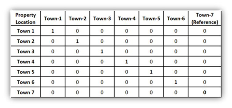
· One category is chosen as the reference (base) category and is represented by all zeros.
· In a jurisdiction with k distinct categories (Towns in our case), we must always create exactly k - 1 dummy variables. Including a dummy variable for every single category creates a mathematical trap known as perfect multicollinearity (or the "dummy variable trap").
In our model:
1. We have 7 towns.
2. We created 6 dummy variables (Town-1 through Town-6).
3. Town-7 serves as the reference category (all dummies = 0).
How to Read the Coefficients:
· The Intercept represents the base Just Value for a property in Town-7 (reference), with all other variables at their baseline.
· Each Town-X coefficient shows the average difference in Just Value for properties in that town compared to Town-7, holding all other characteristics (size, age, bathrooms, PUD, etc.) constant.
Dummy Coding Matrix for the Seven Towns:
1.4 Model Summary Statistics & Coefficients
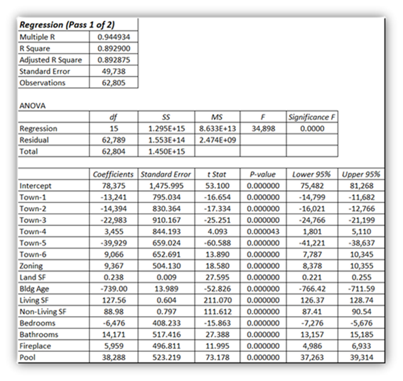
The overall metrics from the Regression output (Pass 1 of 2) demonstrate an incredibly strong baseline model prior to any outlier removal:
· R-Square (0.8929): This indicates that 89.29% of the variance in town-wise Just Values is explained by the foundational and conditional variables inside the pipeline.
· Standard Error ($49,738): The "average miss" of the model is roughly $49.7k. Given the broad range of a countywide property mix, this is low for a first-pass model and will tighten significantly in Pass 2.
· F-Significance (0.0000): The overall F-statistic of 34,898 means the probability that this combination of variables happened by chance is virtually zero.
Physical & Amenity Coefficients
Looking at the coefficients block, we can read the marginal contribution of each physical feature:
· Living SF vs. Non-Living SF: The model adds $127.56 per square foot of heated living area, compared to $88.98 per square foot for non-living spaces (garages, porches, patios).
· Bldg Age (-$739.00): Properties depreciate by exactly $739 per year. For a home at the county's median age of 38, this relatively low annual depreciation reflects strong, sustained demand from the local retiree demographic.
· The Layout Dichotomy (Bedrooms vs. Bathrooms):
o The Bedrooms variable carries a negative coefficient of -$6,476, indicating that when square footage is held constant, carving a house into more bedrooms reduces value—confirming a modern consumer preference for open layouts.
o The Bathrooms variable carries a positive premium of +$14,171, showing a strong willingness to pay for high-utility amenities.
· Zoning & Fixed Features: Being located inside a PUD commands a premium of $9,367 due to neighborhood-specific infrastructure and shared amenities. Adding an in-ground Pool boosts value by $38,288, while a Fireplace adds $5,959.
1.4.1 Reading Town Coefficients Relative to the Intercept
For non-technical assessment personnel, understanding the Intercept is vital. The Intercept ($78,375) represents the theoretical base value of a property when all continuous independent variables are zero, and all dummy-coded categorical variables are set to their reference states.
Crucially, because Town-7 was excluded from the model as the reference baseline, the Intercept inherently represents Town-7's geographic baseline.
The coefficients for Towns 1 through 6 show the direct premium or discount of moving a property to that specific town relative to Town-7:
· Town-1 (-$13,241): A property in Town-1 is worth $13,241 less than an identical property in Town-7.
· Town-2 (-$14,394): Worth $14,394 less than the Town-7 baseline.
· Town-3 (-$22,983): Represents the deepest localized penalty, lagging Town-7 by nearly $23k.
· Town-4 (+$3,455): Commands a positive location premium, lifting values $3,455 above Town-7.
· Town-5 (-$33,929): Slags significantly behind the baseline.
· Town-6 (+$9,066): Represents the strongest premium location among the explicitly coded towns, tracking $9,066 higher than Town-7.
1.4.2 Determining Coefficient Significance
We evaluate each coefficient using four key statistics:
1. t-Stat (absolute value > ~2 is generally significant):
o All variables have very high |t-stats| (e.g., Pool = 73.18, Living SF = 211.07).
2. P-value (< 0.05 = statistically significant):
o Every variable in the model has P-value = 0.0000 (or very close), meaning we are extremely confident the relationships are real and not due to chance.
3. 95% Confidence Interval (Lower & Upper 95%):
o Narrow intervals indicate precise estimates.
o Example: Pool premium is between $37,263 and $39,314 with 95% confidence — very tight and reliable.
o Building Age interval is also very tight around –$739.
4. Standard Error:
o Smaller relative to the coefficient = more reliable.
o Unlike the t-stat or the P-value, there is no absolute, universal rule-of-thumb number for the Standard Error (SE) of a coefficient. This is because the Standard Error is entirely dependent on the scale and unit of measurement of its corresponding independent variable.
Bottom line: This Pass 1 model is already very strong. After applying the 2-Pass Outlier Protocol (removing Z-score outliers beyond ±2 in Pass 2), we expect an even better fit, lower Standard Error, and improved uniformity metrics.
1.4.2 Pass 1 Sample – Under & Over-Valued Properties
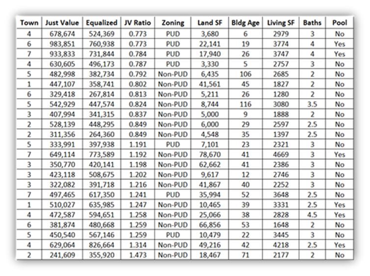
These sample cases demonstrate the severe variance present in Pass 1. The extreme swings are caused by structural anomalies: century-old homes on standard lots with zero redevelopment potential (Town 5, JVR 0.792), or overbuilt houses where massive structural footprints are forced onto tiny suburban lots (Town 4, JVR 0.773).
Left uncorrected, standard OLS regression will warp trying to accommodate these outliers. In Pass 2, we unpack the exact Z-score matrix filters used to isolate these specific failure modes, thereby automatically reducing the global standard error from $49,738 to $35,963.
1.5 Regression Pass 2
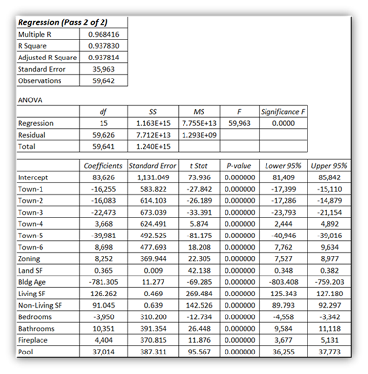
After running Pass 1 on all 62,805 observations, we applied the 2-Pass Outlier Protocol (Z-scores beyond ±2). This removed approximately 5% of the observations (3,163 properties), leaving a cleaner dataset of 59,642 properties for Pass 2.
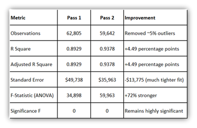
Summary of Key Improvements (Pass 1 → Pass 2)
Interpretation of Improvements:
1. R Square increased to 93.78%: The model now explains 93.78% of the variation in Just Values (up from 89.29%). This is an outstanding fit for a practical Equalization Model using only foundational and conditional variables.
2. Standard Error dropped significantly ($49,738 → $35,963): The average “miss” between the model’s predicted Just Value and the assessor’s Just Value is now much lower. This means predictions are substantially more precise after removing outliers.
3. F-Statistic nearly doubled (34,898 → 59,963): The overall model is even more statistically robust.
4. Coefficient Stability & Precision
o All coefficients retained the same direction (positive or negative), which is a sign of a stable, well-specified model.
o 95% Confidence Intervals are noticeably tighter (more precise estimates).
o All variables remain highly statistically significant (P-value = 0.0000).
Why These Improvements Matter for Equalization Models
Removing outliers via the 2-Pass Protocol eliminates properties that distort the “typical” relationships (e.g., unique luxury homes, distressed properties, or data entry errors). The result is:
· Better uniformity across the roll
· More defensible values when explaining to homeowners or Value Adjustment Boards
· Stronger foundation for Just Value Ratios (JVR) analysis (coming next)
· A model that truly reflects the BLUE (Best Linear Unbiased Estimator) line for our jurisdiction’s Just Values
This is exactly why the 2-Pass Outlier Protocol is a cornerstone of the forensic methodology explained in our recent book, Forensic Valuation Modeling.
1.6 Just Value Ratio (JVR) Analysis: Pre- vs. Post-Outlier Removal
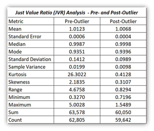
This Just Value Ratio (JVR) analysis summary is the absolute crown jewel of Session 1. It bridges the gap between pure econometric modeling and intuitive mass appraisal equity.
By calculating JVR = Predicted Just Value (Model) ÷ Assessor’s Just Value, we explicitly examine how closely decentralized town assessments align with our mathematically stabilized BLUE baseline.
JVR = Predicted Just Value (Model) ÷ Assessor’s Just Value
JVR = 1.00 → Perfect alignment
JVR > 1.00 → Assessor’s JV underestimated
JVR < 1.00 → Assessor’s JV overestimated
We compare the distribution of JVRs before (Pass 1: 62,805 observations) and after (Pass 2: 59,642 observations), excluding ~5% of observations with Z-scores beyond ±2.
Analysis and Interpretation
1. Central Tendency (Mean & Median) – Major Improvement in Accuracy
The mean JVR moved from 1.0123 to 1.0068 — significantly closer to the ideal value of 1.00. This means the model’s predictions now align much more closely with the assessor’s Just Values on average. The median also improved to nearly 0.9998, showing excellent central alignment after cleaning.
2. Dispersion & Uniformity (Std Dev, Variance, and Range) – Dramatically Better Equity
· Standard Deviation dropped 30% (0.1412 → 0.0989).
· Variance was cut in half.
· The extreme Range collapsed by 82% (4.68 → 0.83).
This is the heart of equalization success: properties are now valued far more uniformly across the jurisdiction.
3. Extreme Values (Min & Max) – Elimination of Wild Outliers
· The worst under-valuations improved from 0.3270 (model says value should be 3x higher) to 0.7196.
· The most extreme over-valuations dropped from 5.0028 (model says value should be 1/4th) to 1.5489.
These extremes were distorting the entire roll. Removing them produces a much more realistic and defensible model.
4. Distribution Shape (Kurtosis & Skewness) – The Most Dramatic Result
· Kurtosis fell from an extremely high 26.30 (very heavy tails / peaked center) to a near-normal 0.41. This collapse shows how just 5% of outliers were creating massive distortion in the dataset.
· Skewness improved from strongly right-skewed (2.18) to mildly skewed (0.31).
Key Insight: A small number of outlier properties (often unusual, unique, or data-error cases) had a disproportionately large negative impact on model performance. The 2-Pass Outlier Protocol successfully restored a much more normal, well-behaved distribution — exactly why this protocol is a cornerstone of forensic valuation modeling.
1.7 Caution: Handling GIS / Spatial Variables (When Available)
The dataset used in this Session is comprehensive, including foundational and conditional variables (location dummies, size, age, bedrooms, bathrooms, amenities, zoning, etc.). However, it does not include GIS or spatial variables (e.g., distance to amenities, neighborhood centroids, flood zones, school district scores, proximity to highways, etc.).
When GIS/Spatial variables are available in your jurisdiction, follow this disciplined approach:
· Introduce them simultaneously during the initial variable selection process, alongside other conditional variables.
· Test them rigorously using the same standards as all other predictors:
o Statistical significance (P-value < 0.05)
o Contribution to model fit without inflating multicollinearity
o Adherence to the principle of parsimony (prefer the simplest model that adequately explains variation)
· They must earn their place in the final model through proper, disciplined selection.
Critical Warning: Do not add GIS or spatial variables “on the fly” later in the process simply to chase better statistics. This common practice often introduces:
· Severe multicollinearity (unstable coefficients)
· Overfitting
· Loss of the BLUE (Best Linear Unbiased Estimator) status
· Models that are hard to explain and defend in appeals or equity hearings
Best Practice Reminder: Stick to the forensic foundation and the disciplined variable-selection methodology as explained in our book, Forensic Valuation Modeling. Spatial variables can be powerful enhancers — but only when introduced properly and thoughtfully from the beginning.
This approach ensures Equalization Models remain transparent, stable, and internally manageable.
1.8 Session Conclusion
Session 1 proves that a highly robust, unassailable Equalization Valuation Model can be built for smaller jurisdictions without relying on vendor software or manual guesswork. By combining Just Value as our fixed-date dependent variable with an objective 2-Pass Regression Protocol, we have successfully converted data chaos into a balanced, tightly bound equity curve. The global metrics are stabilized, the extreme tails are eliminated, and the JVR framework stands ready as an intuitive reporting engine.
Session 1 further proves that a disciplined, Excel-based Equalization Valuation Model can deliver outstanding performance using only standard property characteristics. The jump in model quality after the 2-Pass Outlier Protocol proves why this protocol is foundational.
You now have a repeatable process for building transparent, jurisdiction-controlled models.
1.9 Session Disclaimer
This training module is designed solely for educational, analytical, and system design purposes. The regression models, coefficients, and metrics generated in this masterclass reflect specific data parameters within a controlled research environment. While the methodology is designed to meet high statistical standards, the outputs do not constitute formal, statutory property tax assessments or legal appraisals. Implementation of these protocols within any local jurisdiction must be reviewed against local statutory requirements, administrative codes, and uniform standards of professional mass appraisal practice.
Session 1: How to Run Regression and Descriptive Statistics in Excel (Data Analysis ToolPak)
Important: These instructions assume you are using Microsoft Excel for Windows (Excel 2010 or newer). Mac users can use the free Real Statistics Resource Pack or similar add-ins.
Step 1: Enable the Data Analysis ToolPak (One-Time Setup)
1. Open Excel and go to File → Options.
2. In the Excel Options window, select Add-ins from the left menu.
3. At the bottom, next to “Manage,” select Excel Add-ins and click Go.
4. Check the box for Analysis ToolPak (and Analysis ToolPak – VBA if available).
5. Click OK. → The Data Analysis button should now appear on the Data tab in the ribbon.
Step 2: Running Descriptive Statistics (for JVR Analysis)
1. Prepare your data (e.g., a column containing all the JVR values).
2. Go to the Data tab → Click Data Analysis.
3. Select Descriptive Statistics and click OK.
4. In the dialog box:
o Input Range: Select your JVR column (including header).
o Check Labels in First Row (if you included a header).
o Choose Output Range (select an empty area on the sheet).
o Check the following options:
§ Summary statistics
§ Confidence Level for Mean (optional, default 95%)
§ Kth Largest / Kth Smallest (optional)
§ Click OK.
You will get a full set of statistics, including Mean, Median, Standard Deviation, Kurtosis, Skewness, Range, Minimum, Maximum, etc.
Step 3: Running Multiple Linear Regression (OLS)
1. Organize your data:
o Dependent Variable (Y) = Just Value column
o Independent Variables (X) = All predictor columns (Town dummies, Zoning, Land SF, Bldg Age, Living SF, etc.)
2. Go to Data tab → Data Analysis → Select Regression → OK.
3. In the Regression dialog box:
o Input Y Range: Select the entire Just Value column (including header).
o Input X Range: Select all predictor columns (including headers). Make sure columns are contiguous or select them carefully.
o Check Labels (if headers are included).
o Choose Output Range (select a large empty area — the output is extensive).
o Optional but recommended:
§ Check Residuals
§ Check Residual Plots
§ Check Line Fit Plots
§ Check Normal Probability Plots
o Click OK.
4. Review the output:
o Top section: Multiple R, R Square, Adjusted R Square, Standard Error
o ANOVA table: Overall model significance
o Coefficients table: Individual variable coefficients, t-Stats, P-values, Confidence Intervals
Tip for Pass 2: After removing outliers, repeat the Regression on the cleaned dataset.
Additional Tips for This Series
· Always save a new version of your workbook before running analysis.
· Use Named Ranges or Excel Tables (Ctrl + T) for easier range selection.
· For predictions: After getting coefficients, create a new column using the linear equation: Predicted = Intercept + (Coeff1 × Var1) + (Coeff2 × Var2) + ...
· Document your steps in a separate sheet for audit trails and reproducibility.
These instructions will allow you to replicate everything shown in Session 1 using only standard Excel.
Session 1: Frequently Asked Questions (FAQs)
Q1: What are “Smaller and Mid-Sized Jurisdictions” in this series?
A: For the scope of this series, smaller jurisdictions typically have 50K–100K residential parcels, while mid-sized jurisdictions have 100K–200K parcels. Unlike massive tier-1 metropolitan jurisdictions, these offices typically operate with tighter budgets, limited valuation-modeling staff, and heavy reliance on antiquated legacy vendor software. This masterclass is specifically designed to emancipate these exact jurisdictions.
Q2: What is an Assessment Roll?
A: The Assessment Roll is the official list of all taxable properties in a jurisdiction, including each property’s Just Value (assessed value), owner information, physical characteristics, and location data. It serves as the foundation for property taxation.
Q3: What is Just Value?
A: Just Value (also called Just Market Value, Full Market Value, or Market Value) is the assessor’s estimate of a property’s fair market value as of the valuation date (in this case, 01-01-2026). In this series, Just Value is used as the dependent variable in our models.
Q4: What is an Equalization Valuation Model?
A: An Equalization Valuation Model uses a jurisdiction’s own Just Values (instead of sale prices) as the dependent variable to improve uniformity and equity across the assessment roll. It is a practical, transparent “Crossover” tool between traditional AVM logic and CAMA practices.
Q5: What is the difference between Foundational and Conditional Variables?
A: Foundational variables are core property characteristics that are required by USPAP (Uniform Standards of Professional Appraisal Practice) and therefore stay in the model regardless of their statistical or economic significance (e.g., Land SF must remain even if its P-value > 0.05 or its coefficient is only $2 per square foot).
Conditional variables describe additional property features (e.g., Zoning/PUD, Bathrooms, Bedrooms, Fireplace, Pool) and must justify their place in the model through statistical significance (P-value < 0.05) and adherence to the Principle of Parsimony. Both types are introduced together during disciplined variable selection.
Q6: What is OLS Regression?
A: Ordinary Least Squares (OLS) Regression is the standard statistical method used in Excel’s Data Analysis ToolPak to find the “line of best fit” that minimizes the differences between actual Just Values and model-predicted values. It forms the core engine of our Valuation Models.
Q7: What is the 2-Pass Outlier Protocol?
A: The 2-Pass Outlier Protocol is a disciplined, forensic process developed in our companion books. In Pass 1, we run the model on all data. We then identify and remove statistical outliers (typically Z-scores beyond ±2), and run Pass 2 on the cleaned dataset. This dramatically improves model fit and uniformity, as shown in this session.
Q8: What does achieving “BLUE” status mean?
A: BLUE stands for Best Linear Unbiased Estimator. A model achieves BLUE status when it meets key statistical assumptions (no multicollinearity, unbiased coefficients, minimum variance). Our disciplined approach, including proper dummy coding and avoiding “on-the-fly” variable additions, helps move the model toward BLUE status.
Q9: What is the Principle of Parsimony?
A: The Principle of Parsimony (or Occam’s Razor in modeling) means we prefer the simplest model that adequately explains the data. We retain only variables that are statistically significant and meaningfully improve the model without introducing instability or multicollinearity.
Q10: What is the Just Value Ratio (JVR) and how do we interpret it?
A: The Just Value Ratio is defined as: JVR = Model-Predicted Value ÷ Assessor’s Just Value
JVR = 1.00 → Perfect alignment
JVR > 1.00 → Assessor’s Just Value is underestimated
JVR < 1.00 → Assessor’s Just Value is overestimated
This intuitive ratio is central to measuring uniformity and will be used throughout the series.