
As sea kayakers, our world is governed by the tide. It dictates whether we have a relaxing paddle, an intense session playing in a tidal race, or a grueling fight against a 4-knot conveyor belt. We consult tidal stream atlases, charts, and pilot books to figure out which way the water is moving, when it will turn, and how fast it will run.
But have you ever stopped to wonder where that data actually comes from? How do oceanographers measure a moving, invisible column of water without getting swept away themselves?
The Low-Tech Beginnings: Logs and lines
Measuring the movement of the sea has never been easy. As the 1941 Admiralty Manual of Tides bluntly puts it:
To obtain accurate measurements of the current is not a simple matter…
For centuries, the gold standard wasn't a high-tech sensor, but a method that sounds deceptively primitive. According to a 1978 textbook on ocean tides:
Most of the current speeds and directions on nautical charts have been determined by observing the drift of a special log, weighted to float vertically, from an anchored ship.
While this might sound like guesswork, it was remarkably clever. By weighting a wooden log so that it floated vertically, oceanographers could ensure it bypassed any wind-driven surface effects. Instead, it measured the average current across its entire submerged length. Conveniently, this length could be matched to the draft of a standard ship, giving mariners a useful reading of how the tide would push their vessels.
You can see this exact process captured in photos from the NOAA archive:
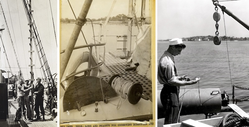 The log has clearly had wood strips added to increase its drag in water, and you can see the line used to measure how far it drifts as the seaman measures the time.
Mechanical marvels
As useful as the log method was, it had glaring limitations. You couldn't leave sailors on an anchored ship throwing logs into the sea every fifteen minutes for months on end to map a few lunar cycles. Oceanographers needed automation.
By the mid-20th century, mechanical current meters emerged, though the Admiralty Manual of Tides noted they came with an entirely new set of headaches:
In all cases the use of a current meter involves many difficulties
Mooring a device in a raging current, keeping it calibrated, preventing the anchored ship's hull from disrupting the water flow, and accurately recording data underwater were massive engineering challenges.
One ingenious mechanical solution used a literal game of marbles. The device featured an impeller (a spinning propeller) turned by the moving water. Inside, a reservoir of steel balls was rigged to drop after a set number of rotations. These balls rolled down a chute aligned with a compass needle, dropping into different compartments based on which way the device was pointing. By counting the balls in each compartment later, scientists could figure out both the speed and the direction of the current!
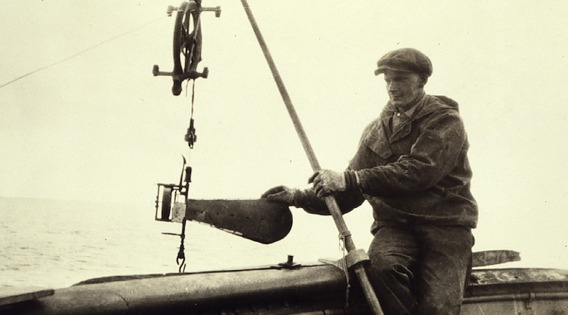 By the mid-1980s, technology progressed to electromagnetic and early acoustic travel-time meters. While more reliable than a game of steel marbles, these devices were still bulky, expensive, and limited to data collection periods of about a year.
Enter the ADCP
Today, the guesswork and marbles are gone. Modern tidal stream data is routinely gathered using an Acoustic Doppler Current Profiler (ADCP). Rather than measuring the water at a single point, these devices map the current across the entire water column simultaneously using sound waves. The tech isn't brand new—the first prototypes appeared in the 1970s—but it became a commercial reality in the 1980s when a company called Rowe-Deines Instruments brought them to market.
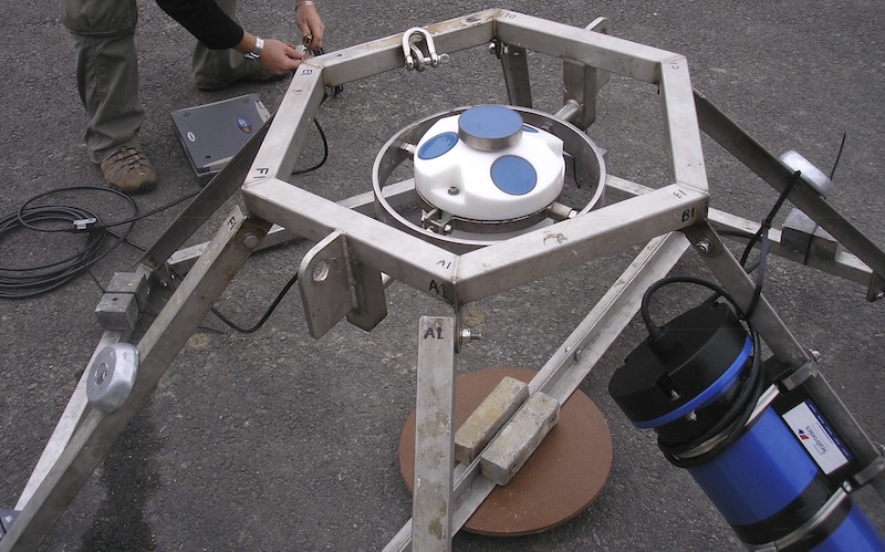 Nortek ADCP (600 kHz AWAC) installed in a frame prior to deployment near The Skerries, Anglesey in 2008. Image: Partrac Ltd, from report "AWAC & ADCP Deployments,Skerries Locations 1-5, 20-27th September 2008
Instead of moving parts, the ADCP relies on high-frequency sound pulses—well above the range of human hearing (typically between 300 to 1200 kHz). The device blasts these sound waves up into the water column. The sound travels through the water until it hits particles suspended in the water—mostly tiny zooplankton, sediment, or air bubbles. These microscopic targets move at the exact same speed as the current and act as acoustic reflectors, bouncing the sound back down to the ADCP's receivers.
The Science: Understanding the Doppler Shift
To calculate water speed from a sound wave, the ADCP relies on the Doppler Effect—the same physics principle that causes a siren to sound high-pitched as an ambulance speeds toward you and low-pitched as it drives away.
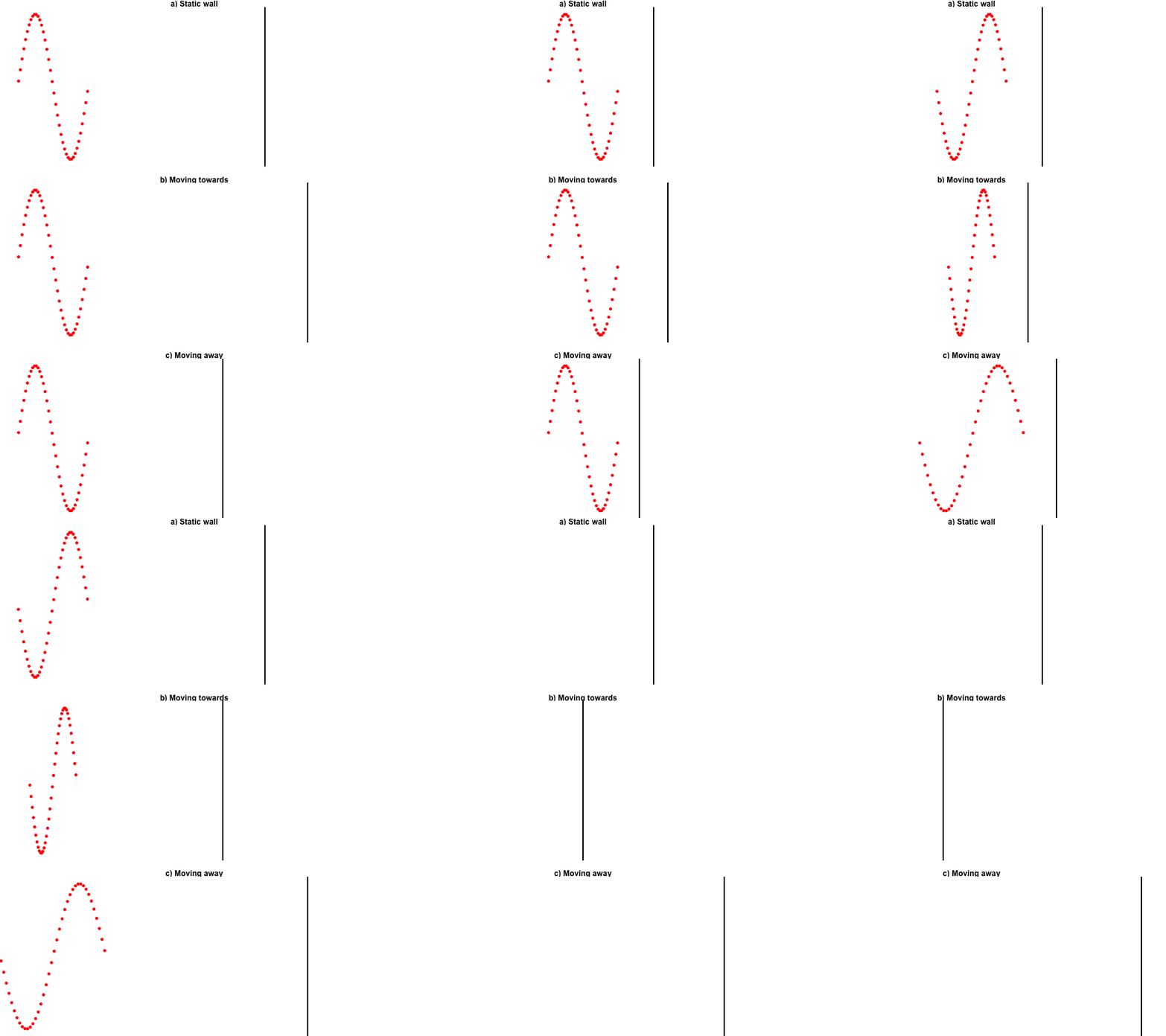
To visualize how this works, imagine a travelling sound wave made up of lots of small particles - I've imagined them as little red bouncy balls in the graphic below. If the wall is completely stationary, the balls bounce off and return to you at the exact same intervals they were thrown ((a) in the diagram below).
Now, what if the object the wave bounces off is moving?:
Moving Toward the Source (b): If the wall is actively moving towards you, it hits the oncoming balls in a shorter time interval than expected. The returning balls are compressed closer together. In acoustic terms, the wavelength shortens, and the frequency increases.
Moving Away from the Source (c): If the wall is moving away from you, the balls take longer to catch up to it and bounce back. The intervals between them stretch out. The wavelength lengthens, and the frequency decreases.
By measuring this change in frequency between the sound pulse it sent out and the echo that returns, the ADCP can instantly calculate exactly how fast the suspended particles (and therefore the water) are moving.
Mapping the Water Column: Beams and Bins
ADCPs are typically anchored flat on the seabed, aiming their acoustic transducers upward toward the surface. Crucially, they don't fire straight up. Instead, they project pulses at fixed angles (usually 20 to 30 degrees from the vertical).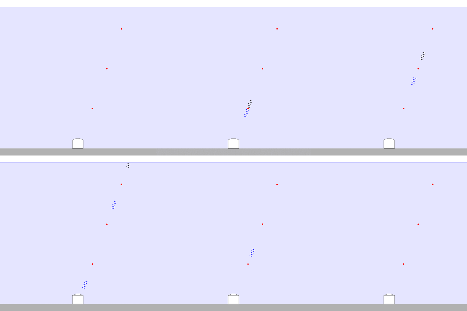 Because sound travels through water at a known, predictable speed (roughly 1,500 meters per second), the ADCP uses time-gating to slice the water column into distinct layers, or 'bins'.
The reflections that return instantly come from the water layers right above the device.
Reflections that take longer to return come from shallower water nearer the surface.
In the animation above, 3 particles are shown at different depths. In reality, there are many particles throughout the water depth, providing a continuous series of reflections. By sorting the returning echoes by time, a single ADCP can map the current speed at (say) 1-meter intervals (or 'bins') from the seabed upwards.
Surfaces and sidelobes
While this sounds perfect, ADCPs have a distinct blind spot right where we sea kayakers are most interested: the surface layers of the water column.
The main acoustic beams are highly focused and narrow, but physics dictates that acoustic transducers also emit weaker rings of energy at wider angles, known as sidelobes.
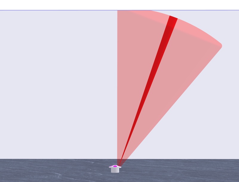 Because these sidelobes travel out at a wider angle, they hit the air-water boundary at the surface before the main, central beam reaches it.
While the sidelobe energy is weak, the water-air interface acts like a giant acoustic mirror, reflecting an incredibly loud echo back to the device. This massive surface echo completely overwhelms (or "swamps") the delicate, quiet reflections coming from the zooplankton in the main beam.
Modern ADCPs have turned this bug into a feature: some models now use those intense surface reflections to track wave heights and capture directional wave data.
Solving the 3D Puzzle
A single acoustic beam can only detect movement along its specific line of sight. It cannot tell if a particle is moving left, right, up, or down—only if it is moving toward or away from the ADCP (red arrows in diagram below).
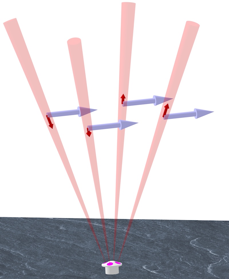 To solve this, ADCPs typically utilize four independent beams pointing in different directions (arranged like an upside-down pyramid). By assuming that the tidal stream (blue arrows) is reasonably uniform across the horizontal span of the beams at any given depth, the device combines the data from all four beams.
Using trigonometry, it calculates the true 3D fluid velocity vector: dividing the flow into North-South, East-West, and Up-Down components. The fourth beam isn't strictly necessary for the math, but it provides a vital data check to make sure that the water isn't too turbulent for a clean reading.
Deciphering the Data
Thanks to universities, environmental agencies, and offshore energy developers, some ADCP data is now preserved in public repositories like the Marine Data Exchange, MEDIN or the British Oceanographic Data Centre.
However, downloading a raw ADCP file isn't like opening a PDF. The files are massive, saved in odd binary formats, and require a fair bit of data-wrangling to extract anything useful.
Worse yet, the internal clocks on deployed ADCPs are prone to drifting over months underwater. Because precise timestamping isn't always critical for academic fluid dynamics, researchers don't always correct it. For a kayaker trying to pinpoint slack water down to the minute, a clock that no one has bothered to correct is unhelpful. Fortunately, ADCPs usually feature built-in pressure sensors. By analyzing the high and low pressure peaks caused by the rise and fall of the tide, we can sometimes reconstruct the true timeline of the data.
So what does the data look like? Here's a plot for some of the data collected by marine consultant Partrac back in 2008 from a location near Carmel Head, Anglesey:
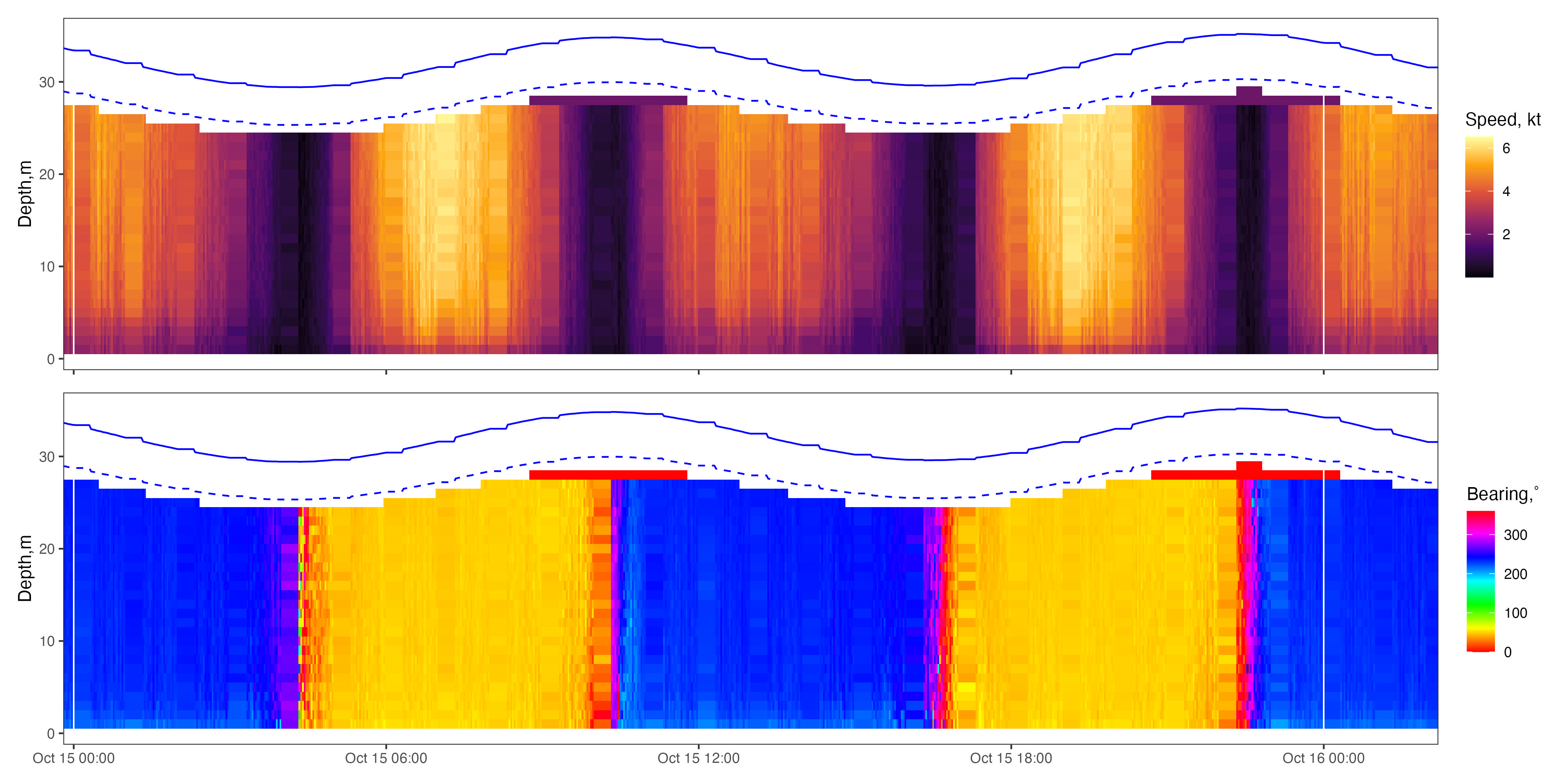 I've extracted about 24 hours worth of data from a day close to springs. There's lots to see in these plots:
The Velocity Profile (Top Plot): The color gradient shows flow speed (yellow high, black low), while the solid blue line tracks the changing depth via the pressure sensor. You can see that slack water here coincides closely with high/low water.
The Surface Blind Spot: See the blank space between the top of the color blocks and the solid blue tide line? That is the sidelobe interference zone. The dashed blue line shows the theoretical cutoff where the data becomes unreliable.
The Raw Power: At peak flow, the stream rages at over 6 knots. Look closely at the vertical profile: the flow is significantly slower near the seabed due to friction (the benthic boundary layer) and fastest in the upper half of the water column. You can also see a clear asymmetry—the flood tide runs noticeably harder than the ebb at this specific location.
The Direction (Bottom Plot): This tracks the compass bearing of the stream. The flood pushes consistently toward the north-east, and the ebb flips around toward the south-west. When the tide turns, it doesn't just stop; it swings briefly through north.
Both plots show a fair bit of noise - as you might expect from a measurement method that relies on reflecting sound off zooplankton, and assumes uniform flow speed in a 6 knot stream. Fortunately, we can average across depths to reduce this noise.
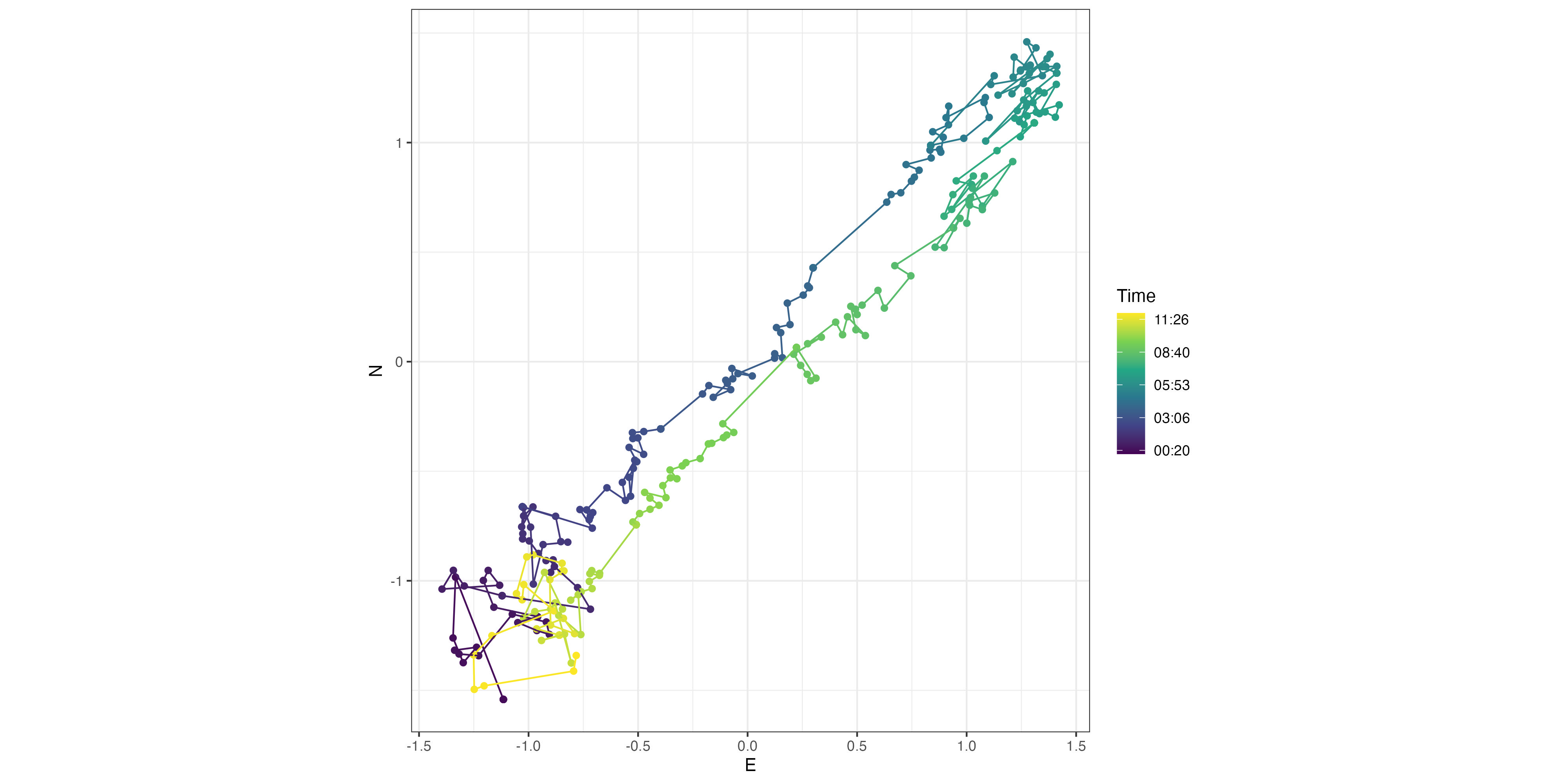 The plot above shows data from a few miles away after depth-averaging has been applied. Each dot represents the water's speed and direction at a single moment over a 12-hour cycle. By extracting the primary axis of the flow (the North-East/South-West highway), we can convert this scatter plot into a clean, classic speed vs. time curve. Here's the data from the first pair of plots above shown in this depth-averaged NE/SW speed vs. time format:
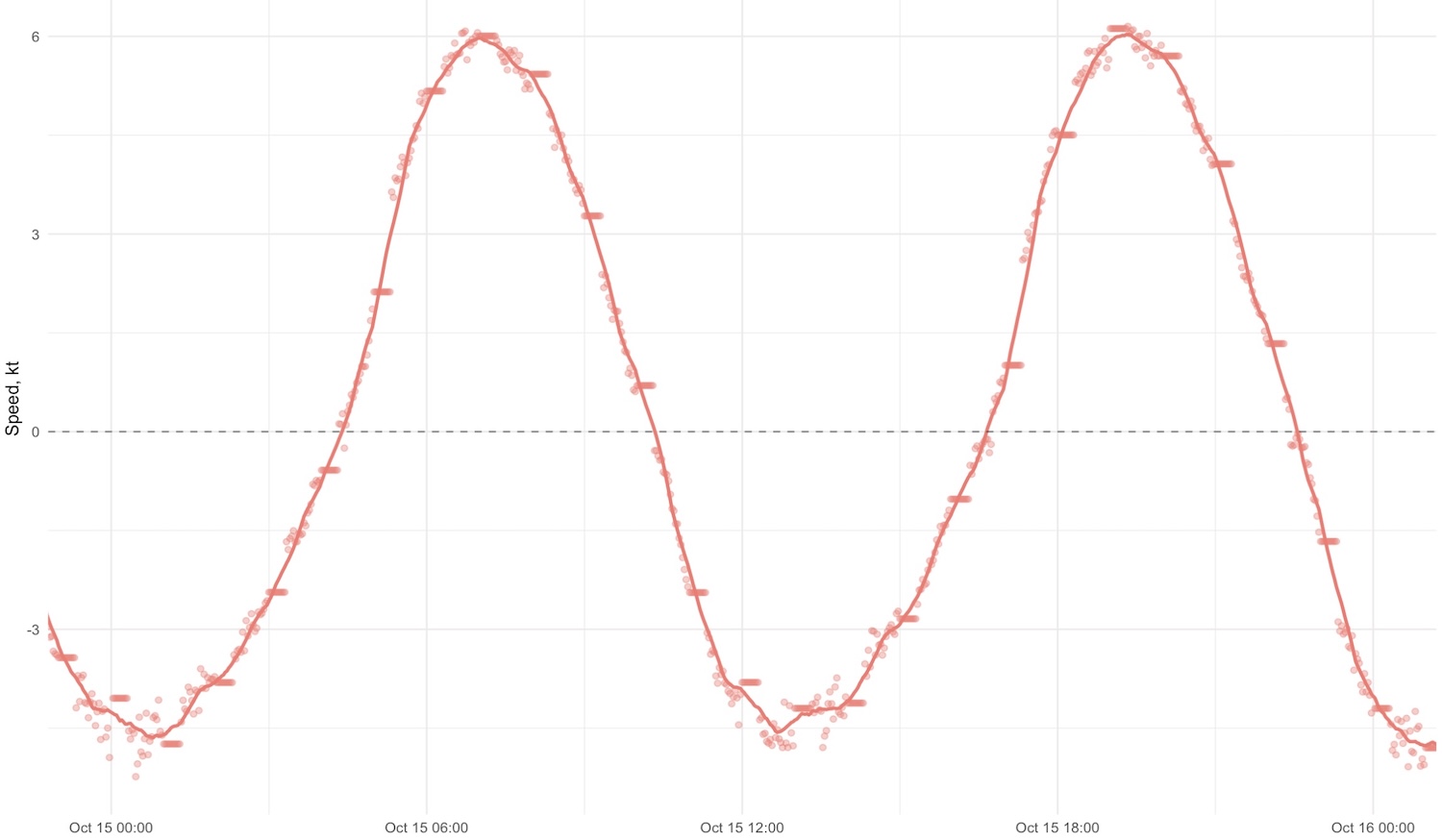 By plotting a mathematically smoothed line through the filtered points, the noise evaporates. Now, we have a highly reliable, precise window into the exact minute of slack water, along with a perfect model of how the current accelerates and decelerates over time. And if the ADCP is in place for a few weeks, as this one was, there's many slack water times that can be compared with a set of tide tables.
A digital future?
Much of the tidal information we use for our planning today on our decks is either purely anecdotal, or measured by sailors watching a wooden log drift away from their anchored ship. ADCPs have changed the game completely. They give us the power to map tidal streams throughout the water column with minute-by-minute precision across entire tidal cycles.
The catch? Deploying these instruments in environments with fast flows remains an expensive, logistically complex task, and the data rarely gets turned into consumer-friendly formats - if it gets released at all. However, as the tidal energy sector expands, the demand for high-resolution ADCP data is increasing. Perhaps if larger volumes of this data become public in the coming years, we'll be able to develop tools to quickly extract the data we need from it - extracting slack water times isn't currently hard to do, it's just a bit tedious. And perhaps we'll finally be to be able to ground some of our planning in decent, verifiable data.