Machine Learning has proven grounds of transformation in recent years, powering everything be it recommendation engines to self-driving cars.

Machine Learning is a type of Artificial Intelligence that works mostly on its own and learn from its experience without being explicitly programmed. But how can you see it in action?

In this article, we’ll break down the essentials of machine learning and demonstrate a practical example of how to build a basic model to solve a real-world problem. But before starting we will look at some basic definitions that we all need to understand in order to work in a particular domain.

Machine learning can be broadly divided into three types:

1. Supervised Learning: The algorithm learns from labeled data, where the input and corresponding output are known.
   For instance, training an algorithm to recognize dogs in images involves feeding it numerous labeled dog images.

2. Unsupervised Learning: The algorithm learns from unlabeled data, identifying patterns and relationships without specific guidance.
   This approach is useful for clustering, anomaly detection, and market basket analysis.

3. Reinforcement Learning: This involves training models through rewards and penalties. It’s commonly used in robotics, gaming, and self-driving cars.

Now let’s get started!

Pre-requisites

1. Python — https://www.python.org/downloads/

2. Jupyter Notebook — https://jupyter.org/install

After installing Jupyter Notebook, you can go to the folder of your choice, right click and then “Open In Terminal” and then run:

jupyter lab

The above instruction is given in doc when you install Jupyter Notebook.

Real-World Example: Predicting Housing Prices

In this example, we would predict the future house prices based on past data like house size, number of bedrooms, locations etc.

Step — 1: Preparing The Data

Data preparation is essential for machine learning. Here, you need a dataset with features (like square footage, number of bedrooms, age of the house, etc.) and a target variable (the house price).

You can download this Excel that has 1000 rows for you to test it further:

https://docs.google.com/spreadsheets/d/1OS72Tr5uR-37dPgFWsvBOQs54wQqPP4izDtafx01FME/edit?usp=sharing

For now, we would be first 4rows to make it simple. This is the data:

Step 2: Selecting and Training a Model

We would be predicting the house prices based on Linear Regression which is a common model for predicting continuous values. Linear Regression finds the best-fitting line that maps inputs (like size, bedrooms, and age) to the target output (price).

This step would mainly focus on three things:

1. Split the data: Divide your dataset into a training set (used to train the model) and a testing set (used to evaluate its accuracy).

2. Train the model: Use the training set to teach the linear regression model. It will determine the relationship between the features and the house price.

3. Test the model: Once trained, use the testing data to see how well the model predicts prices.

Step 3: Implementing the Model in Python

Let’s walk through a basic Python code snippet that demonstrates this process.

To implement we would require some Python libraries for our prediction. These libraries are numpy, pandas, and scikit-learn.

Open your command prompt in the location of your choice and type the following command

pip install numpy pandas scikit-learn

This step would have multiple sub-steps which integrate to model creation of our requirement.

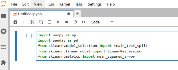
1) Import the packages

Open your Jupyter Notebook. The first step here is to import the necessary packages from the libraries we just installed.

2) Load The Data — DataFrame()

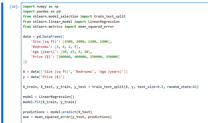
Next, we will load the data we mentioned earlier. To load the data, we would use the DataFrame() of pandas and pass our params like shown below:

These are static data though. At the end of this article, I will show you how to load the entire Excel sheet for implementing the model.

3) Define Features And Set Target Variable

In our case, Features would be Size, Bedrooms, and Age. Which would be the input parameters. And the Price that we want to predict is the Target Variable, or the output parameter.

4) Split The Data

In machine learning, we split the data into training and testing sets (and sometimes a validation set, but not in this case) to ensure that the model we build generalizes well to unseen data.

I have labelled them as:

• Xtrain, ytrain — This shows these are training data

• Xtest, ytest — This shows these are test data

Notice, I’ve written ‘y’ instead Y in y_test — Just machine learning variable tactics 😉

5) Train The Model

This is the crucial part where we would be using LinearRegression` method that would train our model on training data (X_train and y_train) by fitting the model to learn the relationship between the input features (X_train) and the target variable (y_train).

The code looks like this:

6) Testing The Model

Once the LinearRegression has trained our model to predict our house prices, it’s now time to test our work!

• The predict()` of LinearRegression takes our test data to predict the houses.

• The meansquarederror()` takes the y_test` and predictions` as arguments. This method provides a metric to measure the model’s accuracy.

7) Print Our Results!

The final step of writing our code is to print the results that we have trained so far.

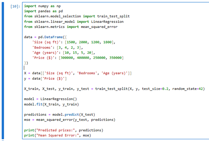
Run your code by pressing the Run button highlighted below

You can also Shift + Enter and see the magic!

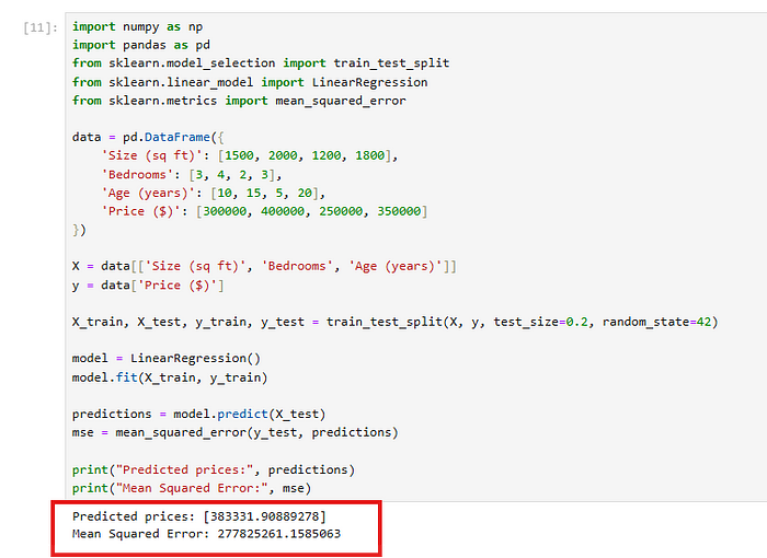
Did you see that?! We just predicted the future cost of our house based on past prices.

The output says:

• Predicted prices: The model predicted a price of approximately $383,331.91 for one of the entries in the test set.

• Mean Squared Error (MSE): The MSE here is 27,782,526.16, indicating the average squared difference between the actual prices and the predicted prices. This indicates that the model’s predictions are closer to the actual values in this case.

A lower MSE indicates a better fit.

Step 4: Evaluating and Improving the Model

This step is require to improve our model to be as close as the required value. If the model’s predictions are not accurate enough, consider improving it by:

• Adding more data

• Engineering new features (e.g., including more neighborhood-related data).

• Trying other models, like Decision Trees or Random Forests. You can also use Feature Scaling, Adding Interaction Terms, Polynomial Regression etc.

Adding more data can help improve the Mean Squared Error (MSE), but it doesn’t guarantee a better MSE always.

Bonus — Load The Excel Sheet As Data Input

Now, in order to improve our model’s performance, we would load the whole Excel sheet that I attached above and then try what the outcome would be.

To load data from an Excel sheet instead of using static values, you can use the pandas library’s read_excel function. Here’s how to modify the code to load data from an Excel file:

data = pd.read_excel('sample_house_data.xlsx', sheet_name='Sheet1')

Note: Try to save your excel sheet in the same location where you have created the Jupyter lab project to learn. This would clutter unnecessary hassle of writing the whole path. If you’ve saved in some other locations in your system, you would need to provide the full path.

You would need to install one more package to deal with Excel sheet in python:

pip install openpyxl

The whole code is shown below:

Ensure the sheet name matches with your excel sheet name.

Thank you for your valuable time to read this 😊

☕ Support My Work on Buy Me a Coffee!

Creating these tutorials and examples takes time and effort, and your support helps me continue making quality content. If you find this helpful, consider buying me a coffee! Every little bit helps and is much appreciated. Thank you! ❤️

🔗 buymeacoffee.com/rohanraobhb